


最新下载
热门教程
- 1
- 2
- 3
- 4
- 5
- 6
- 7
- 8
- 9
- 10
python光学仿真通过菲涅耳公式实现波动模型代码示例
时间:2022-06-25 01:39:26 编辑:袖梨 来源:一聚教程网
本篇文章小编给大家分享一下python光学仿真通过菲涅耳公式实现波动模型代码示例,文章代码介绍的很详细,小编觉得挺不错的,现在分享给大家供大家参考,有需要的小伙伴们可以来看看。
从物理学的机制出发,波动模型相对于光线模型,显然更加接近光的本质;但是从物理学的发展来说,波动光学旨在解决几何光学无法解决的问题,可谓光线模型的一种升级。从编程的角度来说,波动光学在某些情况下可以简单地理解为在光线模型的基础上,引入一个相位项。
波动模型
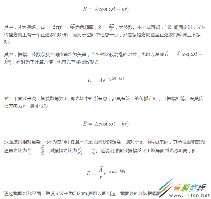
一般来说,三个特征可以确定空间中的波场:频率、振幅和相位,故光波场可表示为:
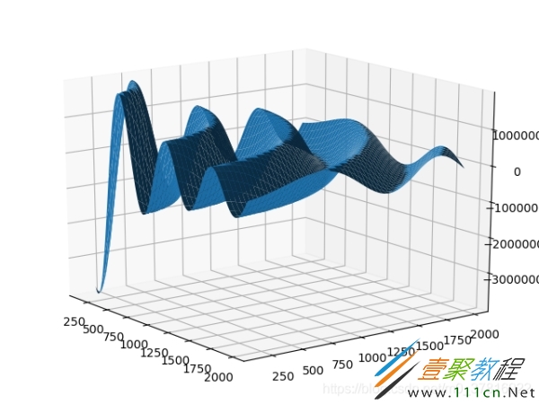
import numpy as np
import matplotlib.pyplot as plt
from mpl_toolkits.mplot3d import Axes3D
z = np.arange(15,200)*10    #单位为nm
x = np.arange(15,200)*10
x,z = np.meshgrid(x,z)      #创建坐标系
E = 1/np.sqrt(x**2+z**2)*np.cos(2*np.pi*np.sqrt(x**2+z**2)/(532*1e-9))
fig = plt.figure()
ax = Axes3D(fig)
ax.plot_surface(x,z,E)
plt.show()
其结果如图所示
菲涅耳公式
几何光学可以通过费马原理得到折射定律,但是无法获知光波的透过率,菲涅耳公式在几何光学的基础上,解决了这个问题。
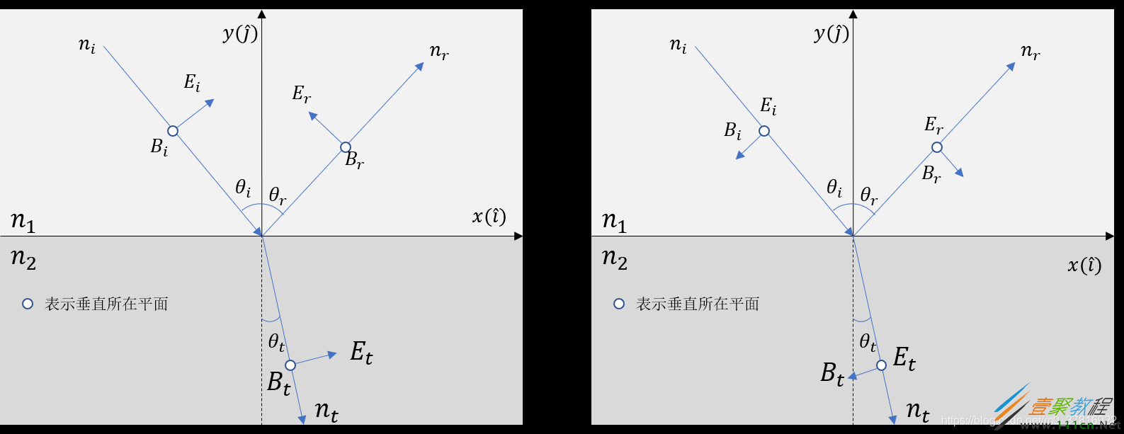
由于光是一群横波的集合,故可以根据其电矢量的震动方向,将其分为平行入射面与垂直入射面的两个分量,分别用p分量和 s 分量来表示。一束光在两介质交界处发生折射,两介质折射率分别为 n1和 n2,对于 p光来说,其电矢量平行于入射面,其磁矢量则垂直于入射面,即只有s分量;而对于 s光来说,则恰恰相反,如图所示。
则对于 p 光来说即
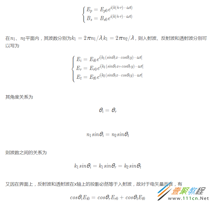
对于磁矢量而言,有
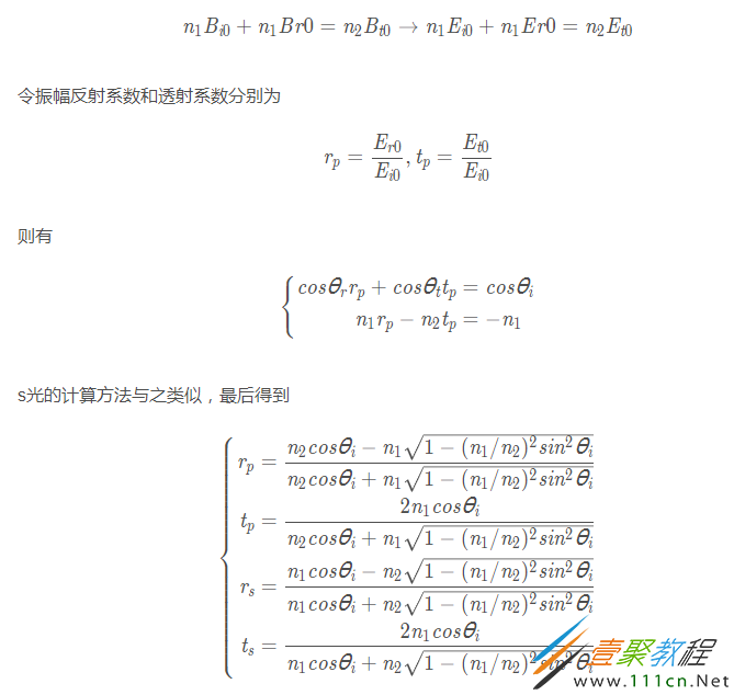
我们可以通过python绘制出当入射光的角度不同时,其振幅反射率和透过率的变化
import matplotlib.pyplot as plt
import numpy as np
def fresnel(theta, n1, n2):
    theta = theta*np.pi/180
    xTheta = np.cos(theta)
    mid = np.sqrt(1-(n1/n2*np.sin(theta))**2)          #中间变量
    rp = (n2*xTheta-n1*mid)/(n2*xTheta+n1*mid)  #p分量振幅反射率
    rs = (n1*xTheta-n2*mid)/(n1*xTheta+n2*mid)
    tp = 2*n1*xTheta/(n2*xTheta+n1*mid)
    ts = 2*n1*xTheta/(n1*xTheta+n2*mid)
    return rp, rs, tp, ts
def testFres(n1=1,n2=1.45):         #默认n2为1.45
    theta = np.arange(0,90,0.1)+0j
    a = theta*np.pi/180
    rp,rs,tp,ts = fresnel(theta,n1,n2)
    fig = plt.figure(1)
    plt.subplot(1,2,1)
    plt.plot(theta,rp,'-',label='rp')
    plt.plot(theta,rs,'-.',label='rs')
    plt.plot(theta,np.abs(rp),'--',label='|rp|')
    plt.plot(theta,np.abs(rs),':',label='|rs|')
    plt.legend()
    plt.subplot(1,2,2)
    plt.plot(theta,tp,'-',label='tp')
    plt.plot(theta,ts,'-.',label='ts')
    plt.plot(theta,np.abs(tp),'--',label='|tp|')
    plt.plot(theta,np.abs(ts),':',label='|ts|')
    plt.legend()
    plt.show()
if __init__=="__main__":
    testFres()
得到其图像为

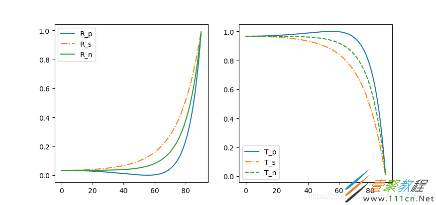
通过python进行绘图,将上面程序中的testFres改为以下代码即可。
def testFres(n1=1,n2=1.45):
    theta = np.arange(0,90,0.1)+0j
    a = theta*np.pi/180
    rp,rs,tp,ts = fml.fresnel(theta,n1,n2)
    Rp = np.abs(rp)**2
    Rs = np.abs(rs)**2
    Rn = (Rp+Rs)/2
    Tp = n2*np.sqrt(1-(n1/n2*np.sin(a))**2)/(n1*np.cos(a))*np.abs(tp)**2
    Ts = n2*np.sqrt(1-(n1/n2*np.sin(a))**2)/(n1*np.cos(a))*np.abs(ts)**2
    Tn = (Tp+Ts)/2
    fig = plt.figure(2)
    plt.subplot(1,2,1)
    plt.plot(theta,Rp,'-',label='R_p')
    plt.plot(theta,Rs,'-.',label='R_s')
    plt.plot(theta,Rn,'-',label='R_n')
    plt.legend()
    plt.subplot(1,2,2)
    plt.plot(theta,Tp,'-',label='T_p')
    plt.plot(theta,Ts,'-.',label='T_s')
    plt.plot(theta,Tn,'--',label='T_n')
    plt.legend()
    plt.show()
得
相关文章
- 代号妖鬼龙宫纯射流玩法攻略 05-22
- 智象未来招聘面试流程怎么走?最新注意事项一览 05-22
- 荒野大镖客2-暴躁老妇人具体位置指南 05-22
- 斗罗大陆诛邪传说双生武魂系统如何解锁 05-22
- 第四届中国AIGC产业峰会怎么参加?2026年参会必备5个步骤 05-22
- 《今古群侠传》传说级武功获取方法全解析:传说级武功实战效果深度剖析 05-22